- 2.1. Introduction
- 2.2. Basic Select
- 2.3. Basic Aggregation
- 2.4. Basic Filter
- 2.5. Basic Filter and Aggregation
- 2.6. Basic Data Window
- 2.7. Basic Data Window and Aggregation
- 2.8. Basic Filter, Data Window and Aggregation
- 2.9. Basic Where-Clause
- 2.10. Basic Time Window and Aggregation
- 2.11. Basic Partitioned Statement
- 2.12. Basic Output-Rate-Limited Statement
- 2.13. Basic Partitioned and Output-Rate-Limited Statement
- 2.14. Basic Named Windows and Tables
- 2.15. Basic Aggregated Statement Types
- 2.16. Basic Match-Recognize Patterns
- 2.17. Basic EPL Patterns
- 2.18. Basic Indexes
- 2.19. Basic Null
For NEsper .NET also see Section J.12, “.NET Basic Concepts”.
Statements are continuous queries that analyze events and time and that detect situations.
You interact with Esper by compiling and deploying modules that contain statements, by sending events and advancing time and by receiving output by means of callbacks or by polling for current results.
Table 2.1. Interacting With Esper
| What | How |
|---|---|
| EPL | First, compile and deploy statements, please refer to Chapter 5, EPL Reference: Clauses,Chapter 15, Compiler Reference and Chapter 16, Runtime Reference. |
| Callbacks | Second, attach executable code that your application provides to receive output, please refer to Table 16.2, “Choices For Receiving Statement Results”. |
| Events | Next, send events using the runtime API, please refer to Section 16.6, “Processing Events and Time Using EPEventService”. |
| Time | Next, advance time using the runtime API or system time, please refer to Section 16.9, “Controlling Time-Keeping”. |
The runtime contains statements like so:
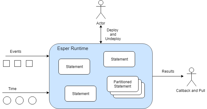
Statements can be partitioned. A partitioned statement can have multiple partitions. For example, there could be partition for each room in a building. For a building with 10 rooms you could have one statement that has 10 partitions. Please refer to Chapter 4, Context and Context Partitions.
A statement that is not partitioned implicitly has one partition. Upon deploying the un-partitioned statement the runtime allocates the single partition. Upon undeploying the un-partitioned statement the runtime destroys the partition.
A partition (or context partition) is where the runtime keeps the state. In the picture above there are three un-partitioned statement and one partitioned statement that has three partitions.
The next sections discuss various easily-understood statements.
The sections illustrate how statements behave, the information that the runtime passes to callbacks (the output) and what information the runtime remembers for statements (the state, all state lives in a partition).
The sample statements assume an event type by name Withdrawal that has account and amount properties.
This statement selects all Withdrawal events.
select * from Withdrawal
Upon a new Withdrawal event arriving, the runtime passes the arriving event, unchanged and the same object reference, to callbacks.
After that the runtime effectively forgets the current event.
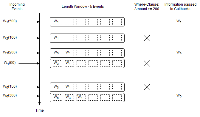
The diagram below shows a series of Withdrawal events (1 to 6) arriving over time.
In the picture the Wn stands for a specific Withdrawal event arriving. The number in parenthesis is the withdrawal amount.
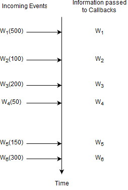
For this statement, the runtime remembers no information and does not remember any events. A statement where the runtime does not need to remember any information at all is a statement without state (a stateless statement).
The term insert stream is a name for the stream of new events that are arriving. The insert stream in this example is the stream of arriving Withdrawal events.
An aggregation function is a function that groups multiple events together to form a single value. Please find more information at Section 10.2, “Aggregation Functions”.
This statement selects a count and a total amount of all Withdrawal events.
select count(*), sum(amount) from Withdrawal
Upon a new Withdrawal event arriving, the runtime increments the count and adds the amount to a running total. It passes the new count and total to callbacks.
After that the runtime effectively forgets the current event and does not remember any events at all, but does remember the current count and total.
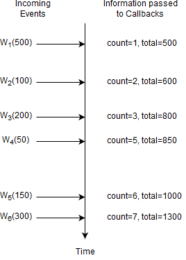
Here, the runtime only remembers the current number of events and the total amount.
The count is a single long-type value and the total is a single double-type value (assuming amount is a double-value, the total can be BigDecimal as applicable).
This statement is not stateless and the state consists of a long-typed value and a double-typed value.
Upon a new Withdrawal event arriving, the runtime increases the count by one and adds the amount to the running total. the runtime does not re-compute the count and total because it does not remember events.
In general, the runtime does not re-compute aggregations (unless otherwise indicated). Instead, the runtime adds (increments, enters, accumulates) data to aggregation state and subtracts (decrements, removes, reduces, decreases) from aggregation state.
Place filter expressions in parenthesis after the event type name. For further information see Section 5.4.1, “Filter-Based Event Streams”.
This statement selects Withdrawal events that have an amount of 200 or higher:
select * from Withdrawal(amount >= 200)
Upon a new Withdrawal event with an amount of 200 or higher arriving, the runtime passes the arriving event to callbacks.
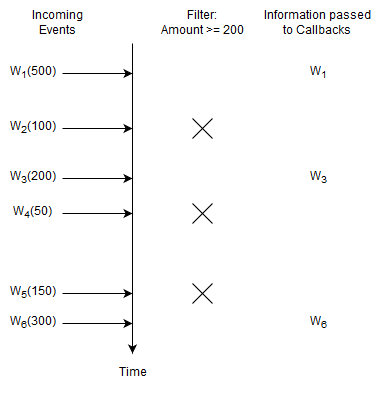
For this statement, the runtime remembers no information and does not remember any events.
You may ask what happens for Withdrawal events with an amount of less than 200. The answer is that the statement itself does not even see such events. This is because the runtime knows to discard such events right away
and the statement does not even know about such events. The runtime discards unneeded events very fast enabled by statement analysis, planning and suitable data structures.
This statement selects the count and the total amount for Withdrawal events that have an amount of 200 or higher:
select count(*), sum(amount) from Withdrawal(amount >= 200)
Upon a new Withdrawal event with an amount of 200 or higher arriving, the runtime increments the count and adds the amount to the running total. The runtime passes the count and total to callbacks.
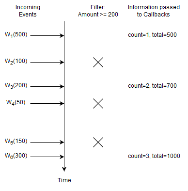
In this example the runtime only remembers the count and total and again does not remember events. The runtime discards Withdrawal events with an amount of less than 200.
A data window, or window for short, retains events for the purpose of aggregation, join, match-recognize patterns, subqueries, iterating via API and output-snapshot. A data window defines which subset of events to retain. For example, a length window keeps the last N events and a time window keeps the last N seconds of events. See Chapter 14, EPL Reference: Data Windows for details.
This statement selects all Withdrawal events and instructs the runtime to remember the last five events.
select * from Withdrawal#length(5)
Upon a new Withdrawal event arriving, the runtime adds the event to the length window. It also passes the same event to callbacks.
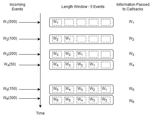
Upon arrival of event W6, event W1 leaves the length window. We use the term expires to say that an event leaves a data window. We use the term remove stream to describe the stream of events leaving a data window.
The runtime remembers up to five events in total (the last five events). At the start of the statement the data window is empty. By itself, keeping the last five events may not sound useful. But in connection with a join, subquery or match-recognize pattern for example a data window tells the runtime which events you want to query.
Note
By default the runtime only delivers the insert stream to listeners and observers. EPL supports optionalistream, irstream and rstream keywords for select- and insert-into clauses to control which streams to deliver, see Section 5.3.7, “Selecting Insert and Remove Stream Events”.
This statement outputs the count and total of the last five Withdrawal events.
select count(*), sum(amount) from Withdrawal#length(5)
Upon a new Withdrawal event arriving, the runtime adds the event to the length window, increases the count by one and adds the amount to the current total amount.
Upon a Withdrawal event leaving the data window, the runtime decreases the count by one and subtracts its amount from the current total amount.
It passes the running count and total to callbacks.
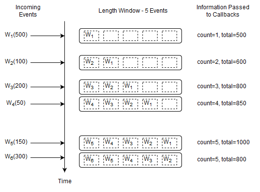
Before the arrival of event W6 the current count is five and the running total amount is 1000. Upon arrival of event W6 the following takes place:
The runtime determines that event W1 leaves the length window.
To account for the new event W6, the runtime increases the count by one and adds 300 to the running total amount.
To account for the expiring event W1, the runtime decreases the count by one and subtracts 500 from the running total amount.
The output is a count of five and a total of 800 as a result of
1000 + 300 - 500.
The runtime adds (increments, enters, accumulates) insert stream events into aggregation state and subtracts (decrements, removes, reduces, decreases) remove stream events from aggregation state. It thus maintains aggregation state in an incremental fashion.
For this statement, once the count reaches 5, the count will always remain at 5.
The information that the runtime remembers for this statement is the last five events and the current long-typed count and double-typed total.
Tip
Use the irstream keyword to receive both the current as well as the previous aggregation value for aggregating statements.
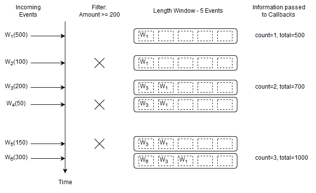
The following statement outputs the count and total of the last five Withdrawal events considering only those Withdrawal events that have an amount of at least 200:
select count(*), sum(amount) from Withdrawal(amount>=200)#length(5)
Upon a new Withdrawal event arriving, and only if that Withdrawal event has an amount of 200 or more, the runtime adds the event to the length window, increases the count by one and adds the amount to the current total amount.
Upon a Withdrawal event leaving the data window, the runtime decreases the count by one and subtracts its amount from the current total amount.
It passes the running count and total to callbacks.
For statements without a data window, the where-clause behaves the same as the filter expressions that are placed in parenthesis.
The following two statements are fully equivalent because of the absence of a data window (the .... means any select-clause expressions):
select .... from Withdrawal(amount > 200)
// equivalent to
select .... from Withdrawal where amount > 200
Note
In EPL, the where-clause is typically used for correlation in a join or subquery. Filter expressions should be placed right after the event type name in parenthesis.
The next statement applies a where-clause to Withdrawal events. Where-clauses are discussed in more detail in Section 5.5, “Specifying Search Conditions: The Where Clause”.
select * from Withdrawal#length(5) where amount >= 200
The where-clause applies to both new events and expiring events. Only events that pass the where-clause are passed to callbacks.
A time window is a data window that extends the specified time interval into the past. More information on time windows can be found at Section 14.3.3, “Time Window (time or win:time)”.
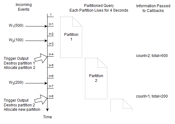
The next statement selects the count and total amount of Withdrawal events considering the last four seconds of events.
select count(*), sum(amount) as total from Withdrawal#time(4)
The diagram starts at a given time t and displays the contents of the time window at t + 4 and t + 5 seconds and so on.
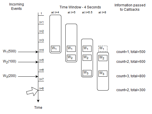
The activity as illustrated by the diagram:
At time
t + 4 secondsan eventW1arrives and the output is a count of one and a total of 500.At time
t + 5 secondsan eventW2arrives and the output is a count of two and a total of 600.At time
t + 6.5 secondsan eventW3arrives and the output is a count of three and a total of 800.At time
t + 8 secondseventW1expires and the output is a count of two and a total of 300.
For this statement the runtime remembers the last four seconds of Withdrawal events as well as the long-typed count and the double-typed total amount.
Tip
Time can have a millisecond or microsecond resolution.
The statements discussed so far are not partitioned. A statement that is not partitioned implicitly has one partition. Upon deploying the un-partitioned statement the runtime allocates the single partition and it destroys the partition when your application undeploys the statement.
A partitioned statement is handy for batch processing, sessions, resetting and start/stop of your analysis. For partitioned statements you must specify a context. A context defines how partitions are allocated and destroyed. Additional information about partitioned statements and contexts can be found at Chapter 4, Context and Context Partitions.
We shall have a single partition that starts immediately and ends after four seconds:
create context Batch4Seconds start @now end after 4 sec
The next statement selects the count and total amount of Withdrawal events that arrived since the last reset (resets are at t, t+4, t+8 as so on), resetting each four seconds:
context Batch4Seconds select count(*), total(amount) from Withdrawal
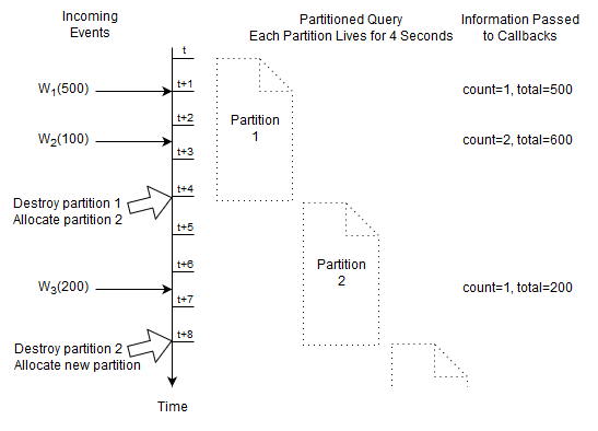
At time t + 4 seconds and t + 8 seconds the runtime destroys the current partition. This discards the current count and running total.
The runtime immediately allocates a new partition and the count and total start fresh at zero.
For this statement the runtime only remembers the count and running total, and the fact how long a partition lives.
All the previous statements had continuous output. In other words, in each of previous statements output occurred as a result of a new event arriving. Use output rate limiting to output when a condition occurs, as described in Section 5.7, “Stabilizing and Controlling Output: The Output Clause”.
The next statement outputs the last count and total of all Withdrawal events every four seconds:
select count(*), total(amount) from Withdrawal output last every 4 seconds
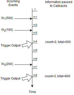
At time t + 4 seconds and t + 8 seconds the runtime outputs the last aggregation values to callbacks.
For this statement the runtime only remembers the count and running total, and the fact when output shall occur.
Use a partitioned statement with output rate limiting to output-and-reset. This allows you to form batches, analyze a batch and then forget all such state in respect to that batch, continuing with the next batch.
The next statement selects the count and total amount of Withdrawal events that arrived within the last four seconds at the end of four seconds, resetting after output:
create context Batch4Seconds start @now end after 4 sec
context Batch4Seconds select count(*), total(amount) from Withdrawal output last when terminated
At time t + 4 seconds and t + 8 seconds the runtime outputs the last aggregation values to callbacks, and resets the current count and total.
For this statement the runtime only remembers the count and running total, and the fact when the output shall occur and how long a partition lives.
Named windows manage a subset of events for use by other statements. They can be selected-from, inserted- into, deleted-from and updated by multiple statements.
Tables are similar to named windows but are organized by primary keys and hold rows and columns. Tables can share aggregation state while named windows only share the subset of events they manage.
The documentation link for both is Chapter 6, EPL Reference: Named Windows and Tables. Named windows and tables can be queried with fire-and-forget queries through the API and also the inward-facing JDBC driver.
Named windows declare a window for holding events, and other statements that have the named window name in the from-clause implicitly aggregate or analyze the same set of events.
This removes the need to declare the same window multiple times for different EPL statements.
The below drawing explains how named windows work.
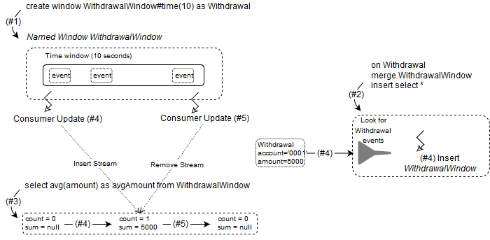
The step #1 creates a named window like so:
create window WithdrawalWindow#time(10) as Withdrawal
The name of the named window is WithdrawalWindow and it will be holding the last 10 seconds of Withdrawal events (#time(10) as Withdrawal).
As a result of step #1 the runtime allocates a named window to hold 10 seconds of Withdrawal events. In the drawing the named window is filled with some events. Normally a named window starts out as an empty window however it looks nicer with some boxes already inside.
The step #2 creates an EPL statement to insert into the named window:
on Withdrawal merge WithdrawalWindow insert select *
This tells the runtime that on arrival of a Withdrawal event it must merge with the WithdrawalWindow and insert the event. The runtime now waits for Withdrawal events to arrive.
The step #3 creates an EPL statement that computes the average withdrawal amount of the subset of events as controlled by the named window:
select avg(amount) as avgAmount from WithdrawalWindow
As a result of step #3 the runtime allocates state to keep a current average. The state consists of a count field and a sum field to compute a running average.
It determines that the named window is currently empty and sets the count to zero and the sum to null (if the named window was filled already it would determine the count and sum by iterating).
Internally, it also registers a consumer callback with the named window to receive inserted and removed events (the insert and remove stream). The callbacks are shown in the drawing as a dotted line.
In step #4 assume a Withdrawal event arrives that has an account number of 0001 and an amount of 5000.
The runtime executes the on Withdrawal merge WithdrawalWindow insert select * and thus adds the event to the time window.
The runtime invokes the insert stream callback for all consumers (dotted line, internally managed callback).
The consumer that computes the average amount receives the callback and the newly-inserted event. It increases the count field by one and increases the sum field by 5000.
The output of the statement is avgAmount as 5000.
In step #5, which occurs 10 seconds after step #4, the Withdrawal event for account 0001 and amount 5000 leaves the time window.
The runtime invokes the remove stream callback for all consumers (dotted line, internally managed callback).
The consumer that computes the average amount receives the callback and the newly-removed event. It decreases the count field by one and sets the sum to null and the count is zero.
The output of the statement is avgAmount as null.
Tables in EPL are not just holders of values of some type. EPL tables are also holders for aggregation state. Aggregations in EPL can be simple aggregations, such as count or average or standard deviation, but can also be much richer
aggregations. Examples of richer aggregations are list of events (window and sorted aggregation) or a count-min-sketch (a set of hash tables that store approximations). Your application can easily extend
and provide its own aggregations.
As table columns can serve as holders for aggregation state, they are a central place for updating and accessing aggregation state to be shared between statements. The below drawing explains how tables work with aggregation state.
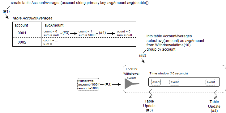
The step #1 creates a table like so:
create table AccountAverages(account string primary key, avgAmount avg(double))
The table that has string-typed account number as the primary key. The table also has a column that contains an average of double-type values. Note how create table does not need to know how the average gets updated,
it only needs to know that the average is an average of double-type values.
As a result of step #1 the runtime allocates a table. In the drawing the table is filled with two rows for two different account numbers 0001 and 0002. Normally a table starts out as an empty table but let's assume the table has rows already.
In order to store an average of double-type values, the runtime must keep a count and a sum. Therefore in the avgAmount column of the table there are fields for count and sum.
For account 0001 let's say there are currently no values and the count is zero and the sum is null.
The step #2 creates an EPL statement that aggregates the last 10 seconds of Withdrawal events:
into table AccountAverages
select avg(amount) as avgAmount
from Withdrawal#time(10)
group by account
The into table tells the compiler to store aggregations not locally as part of the statement, but into the AccountAverages table instead. The as avgAmount tells the compiler to use the column avgAmount in the table.
The compiler checks that aggregation type and value types match with the table column, and that the group by-clause matches the table primary key.
The runtime looks for Withdrawal events and keeps a 10-second time window. Normally a time window starts out as an empty time window but the drawing shows a few events in the time window.
In step #3 assume a Withdrawal event arrives that has an account number of 0001 and an amount of 5000. The runtime adds the event to the time window.
The runtime updates the avgAmount column of the table specifically the two fields count and sum. It increases the count field by one and increases the sum field by 5000.
In the case when a row for the account number does not exist, the runtime allocates a table row and its columns and aggregation fields.
In step #4, which occurs 10 seconds after step #3, the Withdrawal event for account 0001 and amount 5000 leaves the time window.
The runtime updates the avgAmount column of the table. It decreases the count field by one and sets the sum to null as the count is zero.
Other EPL statements may access table columns by putting the table into a from-clause, or by table-access-expression, on-action statement or fire-and-forget query.
The expressions in the select-clause, the use of aggregation functions and the group-by-clause are relevant to statement design. The overview herein is especially relevant to joins, on-trigger, output-rate-limiting and batch data windows.
If your statement only selects aggregation values, the runtime outputs one row (or zero rows in a join).
Without a group-by clause, if your statement selects non-aggregated values along with aggregation values, the runtime outputs a row per event.
With a group-by clause, if your statement selects non-aggregated values that are all in the group-by-clause, the runtime outputs a row per group.
With a group-by clause, if your statement selects non-aggregated values and not all non-aggregated values are in the group-by-clause, the runtime outputs a row per event.
EPL allows each aggregation function to specify its own grouping criteria. Please find further information in Section 5.6.4, “Specifying Grouping for Each Aggregation Function”. The documentation provides output examples for statement types in Appendix A, Output Reference and Samples, and the next sections outlines each statement type.
The examples below assume BankInformationWindow is a named window defined elsewhere.
The examples use a join to illustrate. Joins are further described in Section 5.12, “Joining Event Streams”.
An example statement for the un-aggregated and un-grouped case is as follows:
select * from Withdrawal unidirectional, BankInformationWindow
Upon a Withdrawal event coming in, the number of output rows is the number of rows in the BankInformationWindow.
The appendix provides a complete example including input and output events over time at Section A.2, “Output for Un-Aggregated and Un-Grouped Statements”.
If your statement only selects aggregation values and does not group, your statement may look as the example below:
select sum(amount)
from Withdrawal unidirectional, BankInformationWindow
Upon a Withdrawal event coming in, the number of output rows is always zero or one.
The appendix provides a complete example including input and output events over time at Section A.3, “Output for Fully-Aggregated and Un-Grouped Statements”.
If any aggregation functions specify the group_by parameter and a dimension, for example sum(amount, group_by:account),
the statement executes as an aggregated and grouped statement instead.
If your statement selects non-aggregated properties and aggregation values, and does not group, your statement may be similar to this statement:
select account, sum(amount)
from Withdrawal unidirectional, BankInformationWindow
Upon a Withdrawal event coming in, the number of output rows is the number of rows in the BankInformationWindow.
The appendix provides a complete example including input and output events over time at Section A.4, “Output for Aggregated and Un-Grouped Statements”.
If your statement selects aggregation values and all non-aggregated properties in the select clause are listed in the group by clause, then your statement may look similar to this example:
select account, sum(amount)
from Withdrawal unidirectional, BankInformationWindow
group by account
Upon a Withdrawal event coming in, the number of output rows is one row per unique account number.
The appendix provides a complete example including input and output events over time at Section A.5, “Output for Fully-Aggregated and Grouped Statements”.
If any aggregation functions specify the group_by parameter and a dimension other than group by dimension(s),
for example sum(amount, group_by:accountCategory), the statement executes as an aggregated and grouped statement instead.
If your statement selects non-aggregated properties and aggregation values, and groups only some properties using the group by clause, your statement may look as below:
select account, accountName, sum(amount)
from Withdrawal unidirectional, BankInformationWindow
group by account
Upon a Withdrawal event coming in, the number of output rows is the number of rows in the BankInformationWindow.
The appendix provides a complete example including input and output events over time at Section A.6, “Output for Aggregated and Grouped Statements”.
EPL offers the standardized match-recognize syntax for finding patterns among events. A match-recognize pattern is very similar to a regular-expression pattern.
The below statement is a sample match-recognize pattern. It detects a pattern that may be present in the events held by the named window as declared above. It looks for two immediately-followed events, i.e. with no events in-between for the same origin. The first of the two events must have high priority and the second of the two events must have medium priority.
select * from AlertNamedWindow
  match_recognize (
    partition by origin
    measures a1.origin as origin, a1.alarmNumber as alarmNumber1, a2.alarmNumber as alarmNumber2
    pattern (a1 a2)
    define
      a1 as a1.priority = 'high',
      a2 as a2.priority = 'medium'
)The EPL pattern language is a versatile and expressive syntax for finding time and property relationships between events of many streams.
Event patterns match when an event or multiple events occur that match the pattern's definition, in a bottom-up fashion. Pattern expressions can consist of filter expressions combined with pattern operators. Expressions can contain further nested pattern expressions by including the nested expression(s) in parenthesis.
There are five types of operators:
Operators that control pattern finder creation and termination:
everyLogical operators:
and,or,notTemporal operators that operate on event order:
->(the followed-by operator)Guards are where-conditions that cause termination of pattern subexpressions, such as
timer:withinObservers that observe time events, such as
timer:interval(an interval observer),timer:at(a crontab-like observer)
A sample pattern that alerts on each IBM stock tick with a price greater than 80 and within the next 60 seconds:
every StockTickEvent(symbol="IBM", price>80) where timer:within(60 seconds)
A sample pattern that alerts every five minutes past the hour:
every timer:at(5, *, *, *, *)
A sample pattern that alerts when event A occurs, followed by either event B or event C:
A -> ( B or C)
A pattern where a property of a following event must match a property from the first event:
every a=EventX -> every b=EventY(objectID=a.objectID)
The compliler and runtime, depending on the statements, plan, build and maintain two kinds of indexes: filter indexes and event indexes.
The runtime builds and maintains indexes for efficiency so as to achieve good performance.
The following table compares the two kinds of indexes:
Table 2.2. Kinds of Indexes
| Filter Indexes | Event Indexes | |
|---|---|---|
| Improve the speed of | Matching incoming events to currently-active filters that shall process the event | Lookup of rows |
| Similar to | A structured registry of callbacks; or content-based routing | Database index |
| Index stores values of | Values provided by expressions | Values for certain column(s) |
| Index points to | Currently-active filters | Rows |
| Comparable to | A sieve or a switchboard | An index in a book |
Filter indexes organize filters so that they can be searched efficiently. Filter indexes link back to the statement and partition that the filter(s) come from.
We use the term filter or filter criteria to mean the selection predicate, such as symbol=“google” and price > 200 and volume > 111000.
Statements provide filter criteria in the from-clause, and/or in EPL patterns and/or in context declarations.
Please see Section 5.4.1, “Filter-Based Event Streams”, Section 7.4, “Filter Expressions in Patterns” and Section 4.2.7.1, “Filter Context Condition”.
Filter index building is a result of the compiler analyzing the filter expressions as described in Section 15.18, “Compiler Filter Expression Analysis”. The runtime uses the compiler output to build, maintain and use filter indexes.
Big-O notation scaling information can be found at Section 24.1.1, “Big-O Complexity of Matching Events to Statements and Context Partitions”.
When the runtime receives an event, it consults the filter indexes to determine which statements, if any, must process the event.
The purpose of filter indexes is to enable:
Efficient matching of events to only those statements that need them.
Efficient discarding of events that are not needed by any statement.
Efficient evaluation with best case approximately O(1) to O(log n) i.e. in the best case executes in approximately the same time regardless of the size of the input data set which is the number of active filters.
The runtime builds and maintains separate sets of filter indexes per event type, when such event type occurs in the from-clause or pattern.
Filter indexes are sharable within the same event type filter. Thus various from-clauses and patterns that refer for the same event type can contribute to the same set of filter indexes.
The runtime builds filter indexes in a nested fashion: Filter indexes may contain further filter indexes, forming a tree-like structure, a filter index tree. The nesting of indexes is beyond the introductory discussion provided here.
The from-clause in a statement and, in special cases, also the where-clause provide filter criteria that the compiler analyzes and for which it builds filter indexes.
For example, assume the WithdrawalEvent has an account field. You could create three statements like so:
@name('A') select * from WithdrawalEvent(account = 1)@name('B') select * from WithdrawalEvent(account = 1)@name('C') select * from WithdrawalEvent(account = 2)
In this example, both statement A and statement B register interest in WithdrawalEvent events that have an account value of 1.
Statement C registers interest in WithdrawalEvent events that have an account value of 2.
The below table is a sample filter index for the three statements:
Table 2.3. Sample Filter Index Multi-Statement Example
Value of account | Filter |
|---|---|
1 | Statement A, Statement B |
2 | Statement C |
When a Withdrawal event arrives, the runtime extracts the account and performs a lookup into above table.
If there are no matching rows in the table, for example when the account is 3, the runtime knows that there is no further processing for the event.
For filter index planning, we use the term lookupable-expression to mean the expression providing the filter index lookup value.
In this example there is only one lookupable-expression and that is account.
We use the term value-expression to mean the expression providing the indexed value.
Here there are three value-expressions namely 1 (from statement A), 1 (from statement B) and 2 (from statement C).
We use the term filter-index-operator to mean the type of index such as equals(=), relational (<,>,<=, >=) etc..
As part of a pattern you may specify event types and filter criteria. The compiler analyzes patterns and determines filter criteria for filter index building.
Consider the following example pattern that fires for each WithdrawalEvent that is followed by another WithdrawalEvent for the same account value:
@name('P') select * from pattern [every w1=WithdrawalEvent -> w2=WithdrawalEvent(account = w.account)]
Upon creating the above statement, the runtime starts looking for WithdrawalEvent events. At this time there is only one active filter:
A filter looking for
WithdrawalEventevents regardless of account id.
Assume a WithdrawalEvent Wa for account 1 arrives. The runtime then activates a filter looking for another WithdrawalEvent for account 1.
At this time there are two active filters:
A filter looking for
WithdrawalEventevents regardless of account id.A filter looking for
WithdrawalEvent(account=1)associated tow1=Wa.
Assume another WithdrawalEvent Wb for account 1 arrives. The runtime then activates a filter looking for another WithdrawalEvent for account 1.
At this time there are three active filters:
A filter looking for
WithdrawalEventevents regardless of account id.A filter looking for
WithdrawalEvent(account=1)associated tow1=Wa.A filter looking for
WithdrawalEvent(account=1)associated tow2=Wb.
Assume another WithdrawalEvent Wc for account 2 arrives. The runtime then activates a filter looking for another WithdrawalEvent for account 2.
At this time there are four active filters:
A filter looking for
WithdrawalEventevents regardless of account id.A filter looking for
WithdrawalEvent(account=1)associated tow1=Wa.A filter looking for
WithdrawalEvent(account=1)associated tow1=Wb.A filter looking for
WithdrawalEvent(account=2)associated tow1=Wc.
The below table is a sample filter index for the pattern after the Wa, Wband Wc events arrived:
Table 2.4. Sample Filter Index Pattern Example
Value of account | Filter |
|---|---|
1 | Statement P Pattern w1=Wa, Statement P Pattern w1=Wb |
2 | Statement P Pattern w1=Wc |
When a Withdrawal event arrives, the runtime extracts the account and performs a lookup into above table.
If a matching row is found, the runtime can hand off the event to the relevant pattern subexpressions.
This example is similar to the previous example of multiple statements, but instead it declares a context and associates a single statement to the context.
For example, assume the LoginEvent has an account field. You could declare a context initiated by a LoginEvent for a user:
@name('A') create context UserSession initiated by LoginEvent as loginEvent
By associating the statement to the context you can tell the compiler to analze per LoginEvent, for example:
@name('B') context UserSession select count(*) from WithdrawalEvent(account = context.loginEvent.account)
Upon creating the above two statements, the runtime starts looking for LoginEvent events. At this time there is only one active filter:
A filter looking for
LoginEventevents (any account id).
Assume a LoginEvent La for account 1 arrives. The runtime then activates a context partition of statement B and therefore the filter looking for WithdrawalEvent for account 1.
At this time there are two active filters:
A filter looking for
LoginEventevents (any account id).A filter looking for
WithdrawalEvent(account=1)associated tologinEvent=La.
Assume a LoginEvent Lb for account 1 arrives. The runtime then activates a context partition of statement B and therefore the filter looking for WithdrawalEvent for account 1.
At this time there are three active filters:
A filter looking for
LoginEventevents (any account id).A filter looking for
WithdrawalEvent(account=1)associated tologinEvent=La.A filter looking for
WithdrawalEvent(account=1)associated tologinEvent=Lb.
Assume a LoginEvent Lc for account 2 arrives. The runtime then activates a context partition of statement B and therefore the filter looking for WithdrawalEvent for account 2.
At this time there are four active filters:
A filter looking for
LoginEventevents (any account id).A filter looking for
WithdrawalEvent(account=1)associated tologinEvent=La.A filter looking for
WithdrawalEvent(account=1)associated tologinEvent=Lb.A filter looking for
WithdrawalEvent(account=2)associated tologinEvent=Lc.
The below table is a sample filter index for the three statement context partitions:
Table 2.5. Sample Filter Index Context Example
Value of account | Filter |
|---|---|
1 | Statement B Context Partition #0 loginEvent=La, Statement B Context Partition #1 loginEvent=Lb |
2 | Statement B Context Partition #2 loginEvent=Lc |
When a Withdrawal event arrives, the runtime extracts the account and performs a lookup into above table.
It can then hand of the event directly to the relevant statement context partitions, or ignore the event if no rows are found for a given account id.
Event indexes organize certain columns so that they can be searched efficiently. Event indexes link back to the row that the column(s) come from.
Big-O notation scaling information can be found at Section 24.1.3, “Big-O Complexity of Joins, Subqueries, On-Select, On-Merge, On-Update, On-Delete”.
As event indexes are similar to database indexes, for this discussion, we use the term column to mean a column in a EPL table or named window and to also mean an event property or field. We use the term row to mean a row in an EPL table or named window and to also mean an event.
When the runtime performs statement processing it may use event indexes to find correlated rows efficiently.
The purpose of event indexes is to enable:
Efficient evaluation of subqueries.
Efficient evaluation of joins.
Efficient evaluation of on-action statements.
Efficient evaluation of fire-and-forget queries.
Event index building is a result of the compiler analyzing the where-clause correlation criteria for joins (on-clause for outer joins), subqueries, on-action and fire-and-forget queries.
It is done automatically by the compiler. You may utilize the create index clause to explicitly index named windows and tables. You may utilize query planner hints to influence index building, use and sharing.
EPL and SQL use a three-valued logic: besides true and false, the result of expressions can also be unknown. Three-valued logic is a consequence of supporting null to mark absent data.
If a null value affects the result of a logical expression, the result is neither true nor false but unknown.
A null value basically means “could be anything”. It is therefore impossible to tell whether a comparison to null is true or false.
That’s where the third logical value, unknown, comes in. Unknown means “true or false, depending on the null values”.
The result of each of the following comparisons is therefore null (unknown):
null = 1
null <> 1
null > 1
null = null
Nothing equals null. Not even null equals null because each null could be different.
That’s why EPL has the is null predicate to test whether a value is null or not.
Credit: Above is an excerpt from an online text that can be found at http://modern-sql.com/concept/three-valued-logic.